Questions?
Scalar Line Integral Examples
Monday we saw the definition of a scalar line integral as a Riemann sum of a function’s values along an arbitrary curve times the lengths of short segments of that curve. We also saw a calculationally more practical formula that says the line integral of function f along curve r(t) between t = a and t = b is the regular integral from a to b of f(r(t)) ||r’(t)||.
The Idea
Integrate f(x,y) = x + √y along the curve r(t) = ⟨ t, t2 ⟩, 1 ≤ t ≤ 2.
A good starting place is to find r’(t) and its magnitude:

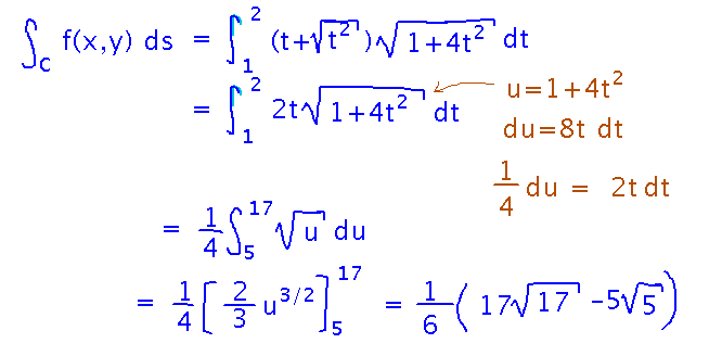
Then you can plug the magnitude into the calculational formula for the line integral, and integrate as a single-variable integral:

A More Complicated Path
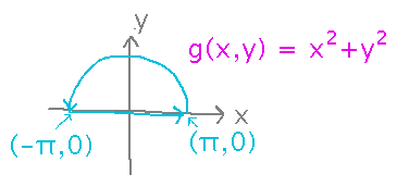
Integrate g(x,y) = x2 + y2 around the path that follows a half circle of radius π from (π,0), above the x axis to (-π,0), then along the x axis back to (π,0):

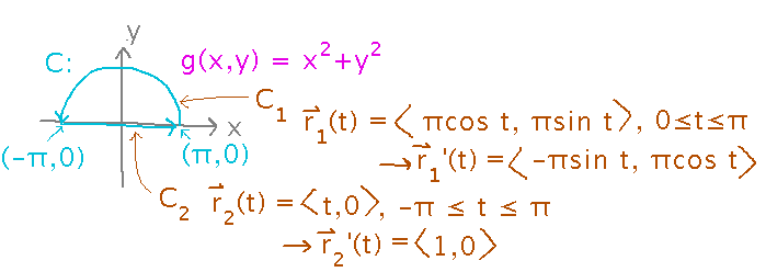
Here we need to treat the path as a piecewise function. We can use a theorem about line integrals that says a line integral over a series of contiguous but non-overlapping paths can be evaluated as the sum of the integrals over the individual paths.

In this case the arc over the top is one subpath and the straight line along the x axis is the another.

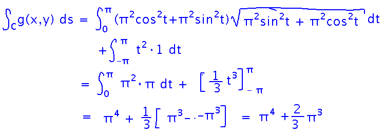
With the subpaths identified and parameterized, plug each into its own integral. Evaluating those integrals is simpler than it might look:

Problem Set
On line integrals and vector fields. We’ve done some of this, but not yet all.
See the handout for details.
Next
Line integrals become more interesting, and more powerfully useful (e.g., in modeling force and work in physics), if the functions you are integrating are themselves vector-valued. Vector valued functions of points in space are called “vector fields.” So let’s learn something about vector fields.
Please read...
- “Examples of Vector Fields”
- “Vector Fields in R2”
- “Drawing a Vector Field”
- The beginning of “Vector Fields in R3”
in section 15.1 of the textbook.
But do not read “Gradient Fields (Conservative Fields)” or beyond (even though it looks like it’s part of “Vector Fields in R3”).