Introduction to Vector Fields

Return to Course Outline

Previous Lecture

Questions?

Vector Fields

First 4-ish subsections of section 15.1.

Key Ideas or Questions

Assign vectors to points in 2D or 3D space.

Widely used to describe such things as force or velocity in modeling the physical world.

2D Example

A vacuum tube was an electronic device that sent electrons through a vacuum between negative and positive electrodes, and could amplify an electrical signal by controlling how easy or hard it was for those electrons to flow. So a very simple vacuum tube looks like a constant-magnitude electrical field between a positive shell and an inner negative electrode:

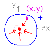
See if we can work out a vector field equation that describes this electric field, at least in a 2-dimensional cross-section through the tube. First, the vectors will point towards the center, because the convention for electric fields is they point in the direction a positive charge would move. Second, we’ve already said that the field has constant magnitude.

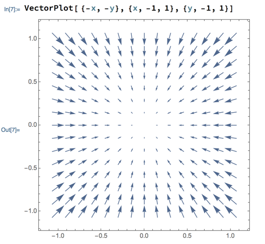
A first step observes that F(x,y) = 〈 -x, -y 〉 points towards the center. But it doesn’t have constant magnitude, magnitudes get smaller with x and y. Plotting the field in Mathematica, using the VectorPlot function, confirms this:

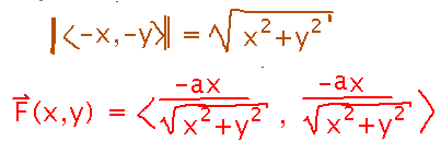
Fix this by scaling the vectors by their magnitudes, to make them unit vectors. And put in a constant of proportionality for units:

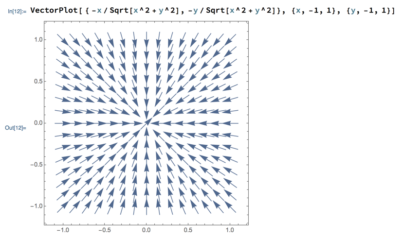
Plotting this looks more like what we intended:

3D Example

See if we can come up with a vector field somewhat like the velocity of water spiraling down a drain. In other words, when viewed from above we want a rotational pattern that gets faster closer to the center, and when viewed from the side we want downward motion that gets more pronounced closer to the center:

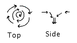
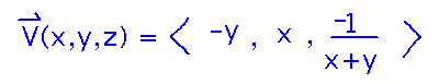
In the x and y dimensions, V(x,y,z) = ⟨ -y, x, ? ⟩ will produce the rotary pattern. In the z dimension, something that approaches -∞ at the origin would be good. Maybe -1/(x+y).

This isn’t very satisfactory when plotted, partly because the z component goes to -∞ when x = y, not just at the origin:

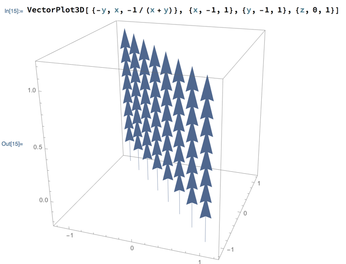
This is a flaw in our thinking about the vector field, but also brings out an awkwardness in Mathematica’s VectorPlot and VectorPlot3D (for 3-dimensional vector fields) functions: they try to normalize the vector lengths they draw to the longest vector, and if that is infinite then all other vectors don’t plot, because they have normalized length 0.

All the Mathematica examples we did today are in this notebook.

Next

Look quickly at a nicer whirlpool vector field.

Mostly line integrals of vector fields.

Please read “Vector Line Integrals” in section 15.2.

Next Lecture