Misc
Scholarships
Geneseo is moving all scholarship management to an online system. Including scholarships selected by the math department.
You need to apply, i.e., get your name into the system, in order to get any scholarship through the college.
Application deadline is March 8.
See https://geneseo.academicworks.com/ for more information.
Problem Set
On arc length and curvature.
See handout for details.
Questions?
Multivariable Functions
Section 13.1.
Key Ideas
Functions with multiple inputs (as opposed to a vector of outputs).
Level curves.
Plotting (with Mathematica or similar technology).
Examples
Lots of things you’ve already seen in math can be described as multivariable functions.
For example, the area of a rectangle, A = hw, can be described as a function A(h,w) = hw.
Other examples?
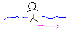
Physics of waves: the amplitude of a wave is a function of both position and time, A(x,t). For instance, a person standing beside a river can stand still and notice waves moving on the river over time, or walk along the river and notice waves rising and falling as position changes:
Force is a function of mass and acceleration: F =ma
Average of x, y, z: A(x,y,z) = (x+y+z)/3. Multivariable functions can have any number of inputs.
A Tangible Example
Think of standing on the ground outside South Hall as standing on the surface of a multivariable function (the function that gives elevation of the ground relative to some reference point).
Level curves are curves in the xy plane along which a multivariable function has a constant value. Compare to contour lines, which are lines at non-zero z along which the function has a constant value. So level curves are contour lines projected into the z = 0 plane. Confusingly, “contour lines” on a topographical (aka contour) map are more like level curves, in that they are curves in a plane that represent lines of constant elevation in a 3D surface.
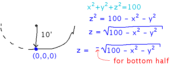
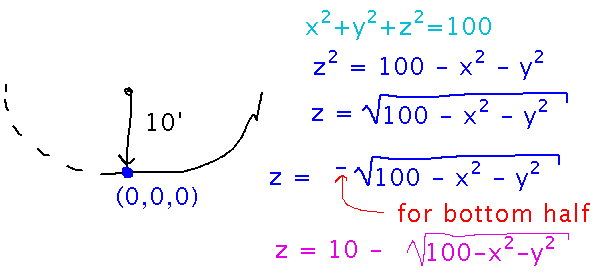
Come up with a function for the “bowl” we were standing in: the bowl is basically a hemisphere, of radius, say, 10 feet. So start with the equation for a sphere, and solve for z, keeping in mind that we want the bottom half of the sphere:
Now remember that the bowl is half a sphere whose center isn’t really at the origin. So we have to offset the hemisphere equation by an amount that puts the center at (0,0,10):
Plotting with Mathematica
Use the Plot3D function.
This notebook demonstrates, on the bowl function we found and another plausible alternative.
Next
Limits of multivariable functions.
Read section 13.2