Introduction to Vector Fields

Return to Course Outline

Previous Lecture

Misc

GREAT Day

Next Tuesday, April 17.

Extra credit for writing a short reaction to any one math-related event (similar to extra credit for colloquia).

Problem Set on Integration

See handout for details.

Questions?

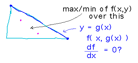
How to handle boundaries in absolute maximum/minimum problems?

Three possibilities have to be considered:

1. An extreme value could occur inside the region you’re searching over. Find critical points by looking for places derivatives are 0 to handle this case.
2. But if the function’s value is generally rising or falling as it crosses a boundary of the region, you won’t have a critical point but could still have an extremum. So check each boundary line separately. To do this, describe the line as a single-variable function (often you can express y as a function of x), and find its critical points as you would for any other single variable function.
3. Finally, the corners of the region won’t necessarily be checked by either of the previous steps, so check each of them explicitly.

Vector Fields

Section 6.1.

Examples

3D

Here’s a vacuum tube, how your grandparents (or great-grandparents) listened to the radio or watched TV.

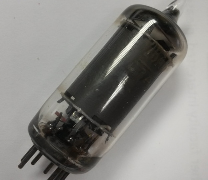
Back before modern electronics, electronic signals were amplified by devices like this, which basically work by creating an electric field in a vacuum, and doing it in a way that lets the field be modulated so that more or less electric current flows through the vacuum. But an electric field has a direction in which it pushes charged particles, and a magnitude (how strongly it pushes), i.e., it’s a vector field!

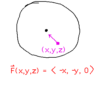
See if you can describe a 3D field in which the vectors have constant magnitude and point towards the z axis (inspired by, if not exactly the same as, the electric field in a vacuum tube).

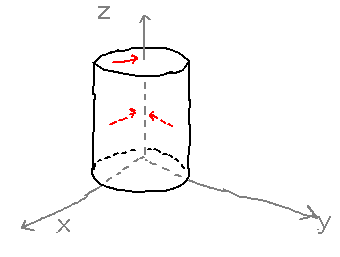
To work out what such a field might be, look down at the tube from the top, and consider how a vector would have to be directed to move a point (x,y,z) towards the z axis (i.e., towards (0,0,z)): The x component of the vector has to be -x and the y component -y, while the z component can be 0. Thus the vector field can be defined by the function F(x,y,z) = 〈 -x, -y, 0 〉.

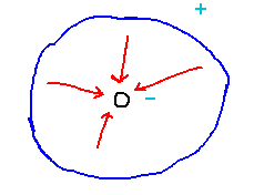
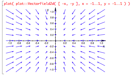
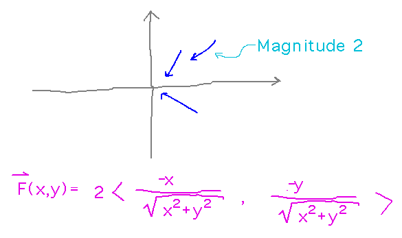
Consider a slightly simpler field: a radial field with all vectors pointing towards the origin in 2D. But all the vectors in that field have length 2. To design this function, start with the idea that vectors of the form〈 -x, -y 〉point towards the origin from point (x,y). But such vectors have different lengths at different distances from the origin, as seen in this muPad plot (which also demonstrates plotting a 2D vector field):

To fix this, divide both components by the vector’s magnitude to get a unit vector. Then multiply the unit vector by 2 to scale it to the desired magnitude:

Plotting Vector Fields with muPad

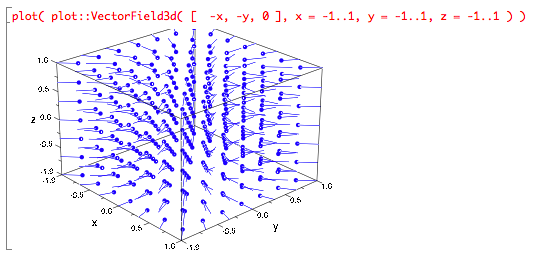
Use the plot::VectorField2d and plot::VectorField3d functions.

For example, here’s a 3D plot of the vector field from the vacuum tube example:

Key Points

The idea of a vector field.

Technology for plotting vector fields.

Next

Introduction to line integrals

Read the “Scalar Line Integrals” subsection of section 6.2.

Next Lecture