SUNY Geneseo Department of Mathematics

Multivariable Functions

Wednesday, February 28

Math 223 04
Spring 2018
Prof. Doug Baldwin

Misc

Colloquium

An Overview of Inverse Problems.

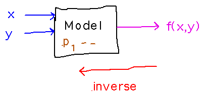
Many mathematical models are essentially functions that take certain inputs and some internal parameters and produce a modeled value for something; this is a “forward” problem. But it’s also common to have a known output, e.g., observed values for a physical system, and want to know what inputs or internal parameters could have produced it; this is the “inverse” problem.

A model produces f(x,y,...) from inputs and internal values; inverse problem takes outputs back to inputs or internal parameters

Sedar Ngoma, Geneseo.

Friday, March 2, 2:30, Newton 203.

Extra credit, as usual.

Questions?

Introduction to Multivariable Functions

Section 4.1

Real-World Examples

See if you can think of some examples of formulas or similar things you know that would count as “multivariable functions”

From Google: temperature as a function of latitude, longitude, and altitude T(Θ, Φ, r)
Waves (simplified form): y(x,t) = sin( x - t )
Kinetic energy in terms of mass and speed: E(m,v) = mv²/2.

These are all “functions” in that they calculate a single number based on arguments, and they are “multivariable” because they have more than one argument variable.

Like single-variable functions, multivariable ones have domains and ranges. For example the domains of the wave and kinetic energy functions above are R² (“R” = reals, “2” denotes pairs; extending this notation, for example, R⁴ would be quadruples of real numbers)

The ranges of the wave and energy functions are [-1,1] and R, respectively.

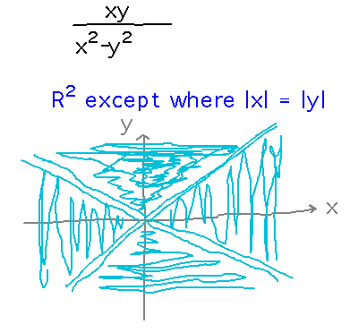
Having 2 dimensions over which arguments can vary means that domains can potentially be more subtly structured than with single-variable functions. For example, consider the function f(x,y) = xy / (x² - y²). Its domain is most of R², except for the two diagonal lines along which |x| = |y|:

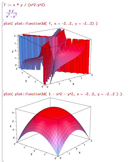
xy plane shaded except along lines x = y and x = -y

Plotting with muPad

Use plot::Function3d to generate a plot object for a function of 2 variables. For example...

Some plots produced by plot::Function2d

Level Curves

What is the equation of the level curve for c = 1 of E(m,v) = mv²/2?

A level curve is simply a curve in the xy plane along which a function has a constant value. In this case it’s E(m,v) = mv²/ 2 that should have a constant value of 1, so the equation for the level curve is mv²/ 2 = 1, or mv² = 2.

This is a fairly simple concept, but widely used to describe 2-variable functions (and analogous things describe functions with more arguments, e.g., level surfaces for 3-variable functions).

Key Ideas

Functions can have more than one argument variable; most of what you know from single-variable functions scales up, although it can become more complicated as it does so.

Level curves as a way to characterize a function’s behavior.

Problem Set

See handout for details.

Limits and continuity for multivariable functions.

Read section 4.2.

Next Lecture