Misc
SI this Afternoon
3:00 - 4:30, Bailey 209.
Problem Set
See handout for details.
Questions?
How to set up the speeding car question from problem set 5?
The basic question is where is a car at time t = 3 seconds if it’s moving at a changing speed, and you know its position at t = 0 seconds.
The key relationship to exploit is that speed is the derivative of distance, and so distance is the antiderivative (integral) of speed. So integrate speed to get distance, and use the known initial distance to find the constant of integration that resulted from the integral.
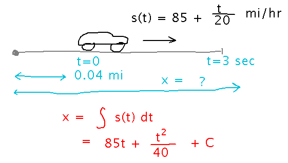
One warning: the problem mixes 2 time units. Sometimes it gives times in seconds, sometimes in hours. So you’ll have to convert between them (using the 1 hour = 3600 seconds equivalence from the problem).
The Mean Value Theorem
Section 4.4.
Warm-Up
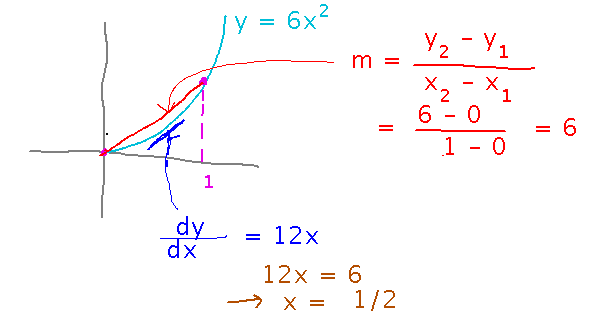
Suppose y = 6x2. What is the value that the Mean Value Theorem says dy/dx must take on between x = 0 and x = 1? Where does dy/dx take on this value?
What the Mean Value Theorem says is that somewhere in the interval 0 to 1 (in this example), the derivative has to be equal to the average (thus “mean” in the theorem’s name) rate of change in y over the interval.
So you can solve this and similar problems by...
- Finding the slope (m) of the line from the left end of the interval, point (x1,y1) (in this case, (0,0)), to the right end, point (x2,y2) ((1,6) here).
- Finding the derivative of the function.
- Setting the derivative equal to m, and solving for x.
Application
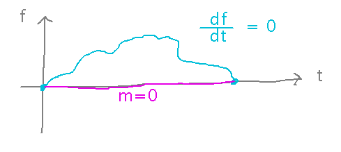
Geneseo’s college flying carpet flies from Geneseo to Rochester and back, taking 1 hour to make the trip. Function f(t), 0 ≤ t ≤ 1, gives the distance between the carpet and Geneseo during the flight, and f’(t) gives the carpet’s speed relative to Geneseo — positive speed means the carpet is receding from Geneseo, negative that it is approaching. Assuming that even a magic flying carpet has a continuous and differentiable distance function f(t), was the carpet’s speed ever 0 at any point other than t = 0 and t = 1 during the trip? Relate your reasoning to the reading.
We don’t know anything about how the carpet’s distance from Geneseo varies with time, except that the distance is 0 when t = 0 and t = 1. But since the slope of the line between those two points on the curve is 0, the Mean Value Theorem says that somewhere on the flight, the derivative of distance, i.e., the speed, was indeed 0.
Consequences
Suppose f′(a) = 0, and for some interval [b,a), f′(x) < 0 while for interval (a,c] f′(x) > 0. Is f(a) a maximum or a minimum?
It’s a minimum, because negative derivative to the left of a means f(x) is decreasing towards f(a), and positive derivative to the right means f(x) is increasing away from it.
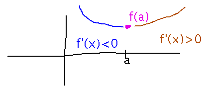
The Mean Value Theorem ensures that a function always decreases over every interval on which it has a negative derivative, and always increases over every interval where the derivative is positive. There’s no possibility of microscopic or localized changes in direction.
Suppose f’(x) = x3 - 2x. Then f(x) could be of the form x4/4 - x2 + C, for any constant C, since all functions of that form have derivatives equal to x3 - 2x. But what, if any, other antiderivatives have we missed?
Another thing the Mean Value Theorem ensures is that we haven’t missed anything — all functions that have the same derivative differ by at most a constant. So our somewhat informal approach to antiderivatives, basically asking “what could have this as its derivative,” is guaranteed to “get it right.”
Next
More estimation of the shapes of graphs, this time using derivative information to find regions where the graph is increasing or decreasing.
Read section 4.5.