Misc
Exam 2
Hour exam 2 is next Monday (November 4).
Covers material up through problem set 8 that wasn’t covered on the first hour exam, i.e., problem sets 6 through 8. Topics include, for example, the chain rule; implicit differentiation; derivatives of exponential, logarithmic, and inverse functions including inverse trig; related rates; extreme values; Mean Value Theorem.
Rules and format similar to first hour exam, especially open-references-closed-person rule.
Extended SI session Thursday, 5:00 - 8:00, Fraser 104.
Sample questions are available in Canvas.
Mid(ish)-Semester Feedback
A chance to give me anonymous feedback on how this course is working.
Return feedback forms by next Wednesday.
Problem Set
...on shapes of graphs and related topics.
See handout for details.
Questions?
Optimization
Section 4.7.
Key Idea(s)
Process for solving optimization problems:
- Identify and name relevant quantities, and find equations relating them. Pay particular attention to what are constraints (often identified in the word problem by “given ...”) and what is the objective function (the thing you want to find a maximum of minimum of).
- Use the constraint to express one independent variable in terms of the other (more generally, if there are more than 2 variables in the constraints, express all but one of them in terms of the other one).
- Write the objective function in terms of that single remaining independent variable.
- Find the optimal (maximum or minimum, according to the problem) value for the objective function; usually this is an absolute maximum or minimum problem, so solve it the same way we solved such problems a few days ago:
- Take the derivative of the objective function.
- Solve for the value(s) of the independent variable that make the derivative 0 (i.e., the critical points).
- Check the endpoints of the interval in which legal values of the independent variable lie (since this is usually an absolute extreme value problem).
- The solution is the critical point or endpoint with the optimal overall value.
Example
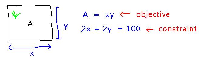
Adapt Example 4.32 to the case where all 4 sides of the garden have to be fenced (maximize area given perimeter is 100 feet).
Start by identifying relevant equations and variables:
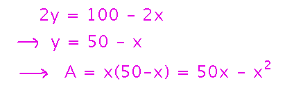
Then express y, and then A, in terms of x:
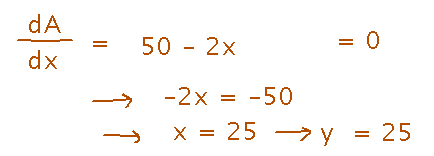
Find critical point(s) for A:
Finally, compare the value of A at the critical point to the values at the smallest and largest possible values for x (0 and 50):
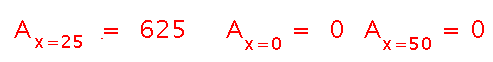
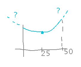
Why look at those endpoints? Because in general we don’t know whether the function curves at those ends in such a way as to make them even better solutions than the critical points (it doesn’t in this example, but could in others):
Flip the Garden Around
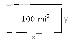
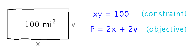
Suppose a rectangular nature preserve needs an area of 100 square miles, with minimum perimeter. What is that minimum perimeter?
Start by identifying constraints and the objective function:
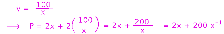
Then express y in terms of x, and then the perimeter in terms of x:
Take the derivative of P:
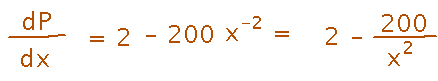
Next
More optimization examples, including finishing the nature preserve problem.