Misc
SI today: 3:00 - 4:30.
Questions?
Inverse trigonometric functions in Mathematica? They generally have names of the form “Arc” (note the capital “A”) followed by the name of the regular trig function, also capitalized. Thus, for example, ArcSin.
See the first line in this notebook for an example.
Problem Set
On implicit differentiation and related rates. See handout for details.
Plotting implicit curves in Mathematica: based on the ContourPlot builtin function.
Here is an example that plots the curve x2 - y2 = 1.
Beware that equality as a relation in Mathematica is two equal signs: ==.
Linear Approximation
Section 4.2.
Key Idea(s)
Use the tangent line to a complicated function at a point as an approximation to the function near that point.
Equation for points (x,y) on the line tangent to f(x) at point (a,f(a)): y = f(a) + f’(a)(x-a)
Applications
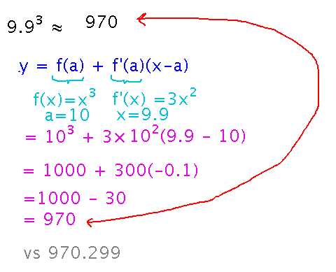
Without using a calculator, estimate what 9.93 is.
Use the tangent line formula, with f(x) = x3, a = 10, x = 9.9:

Suppose traffic radars collect the following information about a particular car:
| Time (Hours) | Distance f/ Start (Miles) | Speed (Miles/Hour) |
|---|---|---|
| 0.5 | 10 | 60 |
| 1.0 | 30 | 45 |
| 1.5 | 25 | -10 |
How far from where it started do you estimate the car was at 1.02 hours?
If you can think of this as data sampled from some largely unknown function and its derivative, you can again use the tangent line formula.
Specifically, think of the main function, f(x), as distance as function of time. Its derivative, f’(x), is then speed.
So now use y = f(a) + f’(a)(x-a), with a = 1 (the time closest to 1.02 at which you have values for the function and its derivative), and x = 1.02. Then y = f(a) + f’(a)(x-a) = 30 + 45(1.02 - 1) = 30 + 45(0.02) = 30 + 0.9 = 30.9
Differentials
Key point: dx, dy, etc. are things meaning an infinitesimally small change in x. This can provide good intuition for lots of notation in calculus, e.g., why dy/dx is a slope. But it breaks down if you look too deeply into what “infinitesimally small” means formally -- limits are a better tool for that formalism.
Next
Start extreme values (i.e., maximums and minimums) of functions.
Read section 4.3 of the textbook.