Continuity

Return to Course Outline

Previous Lecture

Questions?

Continuity

Section 2.4

Key Ideas

Function f is continuous at a if f(a) equals lim_x→a f(x). Which also requires that f(a) and lim_x→a f(x) are defined.

3 types of discontinuity: jump, infinite, removable.

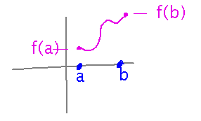
The Intermediate Value Theorem. If f is continuous between a and b, then f(x) “hits” every value between f(a) and f(b):

Example 1

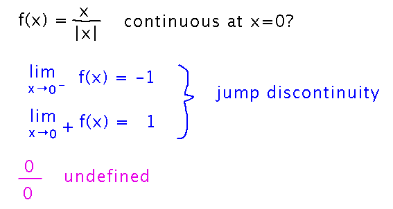
Is f(x) = x / |x| continuous at x = 0? Why or why not?

No, because its limits as x approaches 0 from the left and right differ, so the 2-sided limit doesn’t exist (and there’s a jump discontinuity). It also fails the continuity requirement that f(a) exist in the first place.

More Complicated Example

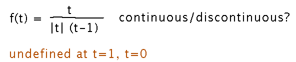
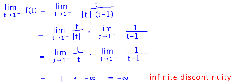
Where is f(t) = t / (|t|(t-1)) continuous? At places where it is discontinuous, what kind of discontinuities does it have?

First, notice that f(t) will be undefined at t=1 because (t-1) is 0 there, and at t=0, because |t| is 0 there. These are the only places where f can be undefined.

So we know the function is discontinuous at those places, but not what sort of discontinuity occurs. For that we need limits....

First, analyze the limits at t = 1. We could try to do this by tabulating some values of f(t), although we would eventually need values on each side of 0, and on each side of 1, to get a feel for how the discontinuities work. And there’s always the danger that we’d miss something important by not picking the right numbers to look at.

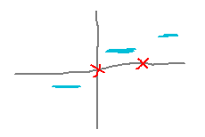
A more rigorous and reliable approach is to find the limits analytically, i.e, via algebra, limit laws, infinite limit theorem, etc. By inspection, it looks like one of the rules from the infinite limit theorem will apply, so let’s try to work in that direction. As soon as we find even one 1-sided limit that is infinite we’ll have met the requirements for an infinite discontinuity.

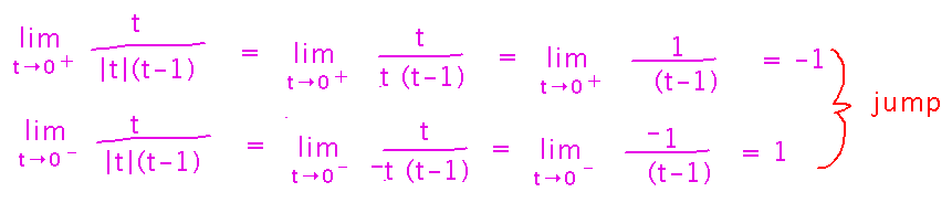
Around t = 0, we need to look at the limits from both sides. Knowing the sign of t lets us simplify the absolute value operation, and the rest is just limit laws. Since both limits exist but aren’t equal, we have a jump discontinuity.

Everywhere except t=0 and t=1, f(t) is continuous. Verify this by noting that f is defined at all these places, a, and that limit laws apply (after simplifying |t| based on whether t is positive or negative), which means that lim_t→a f(t) exists and can be computed by just plugging a into the definition of f, which will necessarily give lim_t→a f(t) = f(a).

Problem Set

See handout for details.

Next

Introduction to derivatives.

How can you use these things you now know about limits to address that rate-of-change aka slope-of-tangent problem from the introduction to this course?

Read section 3.1.

Next Lecture