Introduction to Lagrange Multipliers

Return to Course Outline

Previous Lecture

Questions?

Finishing Absolute Extreme Values

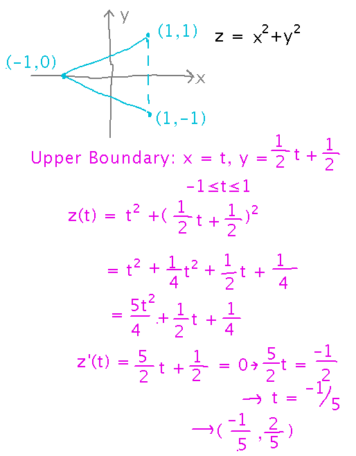
Yesterday we looked for absolute extreme values of z = x² + y² in the xy triangle with vertices (-1,0), (1,1), and (1,-1), and we found a number of candidates. I also think we slipped up with some algebra along the boundary sides from (-1,0) to (1,1) and (-1,0) to (1,-1). Since these are symmetrical, let’s redo one of them carefully:

Now we have a number of candidate locations for the absolute minimum and maximum:

• At the one critical point (0,0), where z = 0
• Along the boundary of the region, at
  • (-1/5,-2/5), where z = 1/5 = 0.2
  • (1,0), where z = 1
  • (-1/5,2/5), where z = 1/25 + 4/25 =1/5 = 0.2
• At the corners of the region, namely
  • (-1,0), where z = 1
  • (1,1), where z = 2
  • (1,-1), where z = 2

So the absolute minimum is 0 at (0,0) and the maximum is 2 at (1,1) and (1,-1).Notice that there’s nothing wrong with a maximum or minimum occurring at multiple points.

Lagrange Multipliers

Section 13.8 in the book

Key Idea(s)

Why this weird formula involving two gradients being multiples of each other? The proof in the book gives all the details, but here are the core ideas: think of the objective function (the one you want to maximize or minimize) and the constraint in terms of their level curves. For the objective function, you want to position x and y on the level curve that has the highest value. But thanks to the constraint, you can’t necessarily do this. Instead, you also have to position x and y on a specific level curve of the constraint function. It turns out that the way to do this while optimizing the objective function is to pick a level curve for the objective function that is tangent to the level curve for the constraint, and pick (x,y) to be the point of tangency. One of the properties of gradients is that they are perpendicular to level curves, so where these two level curves are tangent to each other, their gradients are parallel, i.e., the gradients are scalar multiples of each other. Thus the formula on which Lagrange multipliers are based.

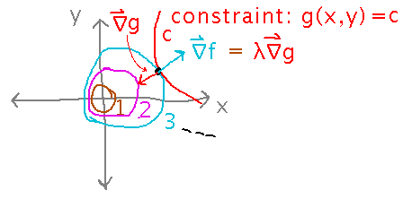
The optimal value of f(x,y,...) subject to constraint g(x,y,...) = c happens when grad f is a scalar multiple of grad g, which gives you equations to solve for x, y, etc.

Example

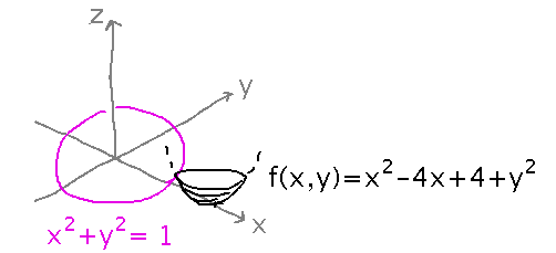
The example I put in the class notes from yesterday to introduce “constrained optimization” was finding a maximum value of f(x,y) = x² - 4x + 4 + y², subject to the constraint that the point (x,y) lies on the circle x² + y² = 1.

Try solving that with Lagrange multipliers.

Question: how do you reconcile the fact that the objective function is given by an explicit equation, whereas the constraint is typically an implicit one? The method has sort of a hack for dealing with this, namely it rephrases the constraint in terms of some function g(x,y) being 0. So in our case where the constraint is the equation x² + y² = 1, the Lagrange multiplier method rewrites this as g(x,y) = x² + y² - 1, i.e., a function that is 0 when x² + y² = 1. But now you have the constraint as a function you can take a gradient of.

Based on this idea, start by writing the constraint function g(x,y), then find gradients and put them into the Lagrange multiplier equation:

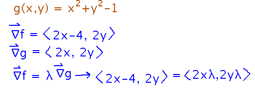
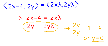
In order for the Lagrange multiplier equation to hold, individual components of the vectors on each side must be equal. This (plus the constraint equation) creates a system of equations you can solve for x and y. But unlike systems of equations in many other contexts, these aren’t necessarily linear, and they don’t necessarily have a nice procedure for finding a solution. It takes more problem-specific cleverness to solve these systems.

And particularly beware of one thing: any time you divide by a variable, you are implicitly assuming that variable is not 0. Make a note that in fact the variable might be 0! Otherwise you “divided away” a solution where it is.

Next

Finish this example and look at another one.

No new reading.

Next Lecture