The Gradient

Return to Course Outline

Previous Lecture

Misc

Another extra credit opportunity: the “extreme values of multivariable functions” discussion is extra credit and available until the day we discuss extreme values in class (probably Monday).

Make half hour appointments next week to grade problem set 10. Experience grading this week suggests that things will go more smoothly, but maybe not fit in 15 minutes yet. They should fit in 2 days though, you all did that very comfortably this week.

Is it helpful for me to post announcements ahead of time as class outlines become available?

Questions?

In the hill example from yesterday, the directional derivative tells you how fast your altitude changes as you walk in the given direction? Yes, exactly.

Gradients

The last 3 subsections in section 13.6 of the textbook.

Key Idea(s)

The gradient is a vector-valued function whose components are derivatives of a multivariable function.

This is the first time we’ve seen a “vector field,” i.e., a vector-valued function with multivariable components.

Applications of the gradient

• A way to compute directional derivatives in terms of gradients
• The gradient points in the direction of greatest change, i.e., the direction in which to change the inputs to a function in order to produce the fastest change in the function’s value.

Basic Idea

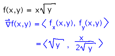
Find ∇f(x,y), given f(x,y) = x √ y.

Plug the derivatives of f with respect to x and y into the definition of the gradient:

What about ∇g(x,y,z,w), where g(x,y,z,w) = x siny - y cosz + ze^w - w lnx?

The idea of gradient as a vector of partial derivatives extends to any number of dimensions/variables. So here, calculate 4 partial derivatives and make a vector from them:

Applications

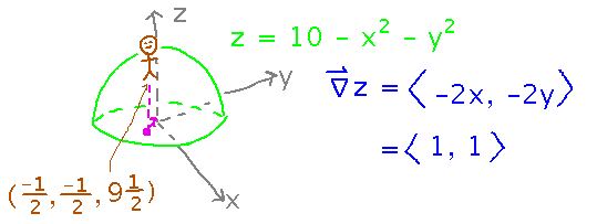
Recall the hill from yesterday, with elevation z = 10 - x² - y², and a person standing at (-1/2, -1/2, 9 1/2) on it. What direction should that person walk in order to ascend fastest towards the top?

Use the idea that the gradient points in the direction of greatest/fastest change: the gradient of z, evaluated at x = -1/2, y = -1/2, will be the direction the person should walk:

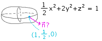
When a video game or computer graphics program draws 3-dimensional shapes, it needs to know normal vectors to them in order to light them realistically. So consider the ellipsoid 1/2 x² + 2y² + z² = 1, and find such a normal vector at point (1, 1/2, 0).

We didn’t have time to finish this problem, but it illustrates another important application of gradients. The book tells you that gradients are perpendicular (normal) to level curves. What it doesn’t tell you is that an implicit surface such as this ellipsoid is a “level surface” for a 3-variable function. In other words, the ellipsoid is the set of points on which the function f(x,y,z) = 1/2 x² + 2y² + z² happens to have the value 1. So the gradient of f will point in the direction perpendicular to that surface, i.e., normal to the ellipsoid.

We’ll probably finish this problem as part of the next problem set.

Next

In the so-called method of Lagrange multipliers, gradients play an elegant role in certain multivariable optimization problems (i.e., problems involving finding values for multiple variables that maximize or minimize some function). So the last thing I want to do with multivariable functions and their derivatives is look at minima, maxima, and optimization.

Via the online extreme values discussion, we’ve already established the key idea for identifying local minima and maxima, namely looking for critical points, places where all the partial derivatives of a function are 0.

Monday, I want to quickly review this, look at a way of telling whether critical points really correspond to extreme values as opposed to so-called “saddle points,” and talk (or start talking) about absolute extreme values.

Please read section 13.7 in the book.

Next Lecture