Misc
Final Exam
Tuesday, May 8, 12:00 noon to 3:20 PM, in our regular classroom.
Comprehensive, but with an emphasis on material since the 2nd hour exam (e.g., directional derivatives, gradients, Lagrange multipliers, multiple integrals & their applications, line integrals, vector fields, etc.)
Designed to be 2 to 2 1/2 times as long as the hour exams, but you have 4 times as much time.
Rules and format otherwise similar to hour exams, particularly including the open-references rule.
I’ll provide a sample from a past semester.
I’ll bring donuts and cider.
SOFIs
No-one has filled one out yet (as of this morning)!
They are useful to me in improving courses for the future, and you get 1 printer dollar / SOFI. So please fill them out.
Questions?
Why does Green’s theorem require integrating around a counterclockwise curve? Basically it’s a convention to respect the fact that the orientation of the curve determines the sign of the line integral, whereas the region over which Green says you can evaluate a multiple integral has no notion of two directions for its boundary.
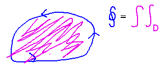
Green’s Theorem
Section 6.4.
Sanity Check
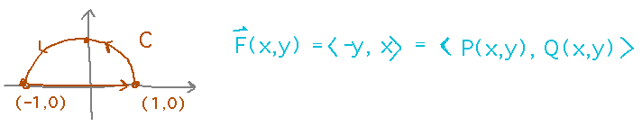
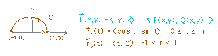
Check that Green’s theorem and the standard line integrals for circulation and flux give the same answers for the circulation and flux of F(x,y) = 〈 -y, x 〉around the semicircle of radius 1 above the origin.
We decided to start by calculating the multiple integral for circulation from Green’s theorem. This needs the derivatives of the components of F. Also notice that since those derivatives are constants, the double integral turns out to be just the area of the semicircle, and so can be calculated geometrically without explicitly evaluating a pair of integrals.
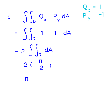
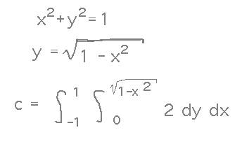
...but if you do want to evaluate the integrals explicitly you can. Doing it in polar coordinates will probably be easier than rectangular.
Checking that this double integral produced the same value as the circulation line integral is a logical next step. To do this, we need parametric forms for the curve. Note that the curve has 2 parts, so we need parametric forms for both:
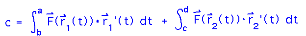
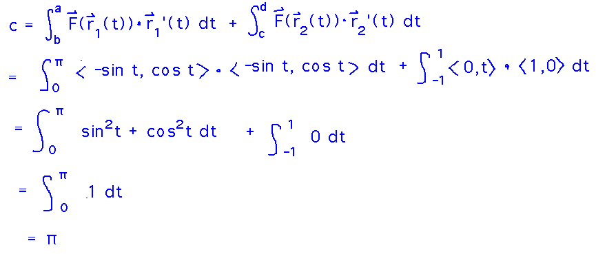
Evaluate the circulation line integral over both paths and add the results to get total circulation:
Do this by expanding the F(r(t)) and r’(t) terms:
Key Points
Working with Green’s theorem.
Green’s theorem as an easier way to evaluate line integrals.
Next
Continue with Green’s theorem, in particular the flux form, looking at equivalences between line integrals in light of it, and applying it to find areas.
No new reading.