Misc
Exam 2 is tomorrow (Thursday).
Questions?
Lagrange Multipliers
Example
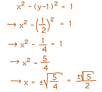
Find the point(s) on the hyperbola x2 - (y-1)2 = 1 that are closest to the origin.
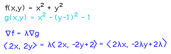
In other words, minimize the distance from the origin (or its square, x2 + y2) subject to the constraint x2 - (y-1)2 = 1. In optimization terminology, the objective function, aka f(x,y) in the book’s discussion of Lagrange multipliers, is f(x,y) = x2 + y2, and the constraint function, g(x,y) in the book, is g(x,y) = x2 - (y-1)2 - 1 (note that this has to be phrased in such a way that the constraint is g(x,y) = 0).
With these identified, the key equation is the relationship between the gradients of f and g:
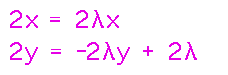
The fact that both components of the gradients have to be equal simultaneously produces a system of equations to solve.
Unlike systems that come up in other contexts, this one isn’t linear, and it has more variables than equations (although you can use the constraint equation to help with this last point). So solving it takes a certain amount of creativity, and may follow different processes for different problems.
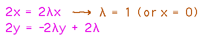
In this case, a good way to start is to use the first equation to deduce that λ = 1. Or more accurately, since that deduction involves dividing both sides of the equation by x, that either λ = 1 or x = 0; but x = 0 isn’t a valid solution because no point on the hyperbola has an x coordinate of 0. In general, be alert for places where algebra leads you to divide by something that might be 0.
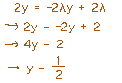
Now we can plug the value for λ into the equation involving y, to solve for y:
Finally, plug the value for y into the constraint equation to find x:
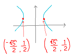
So the closest points on the hyperbola to the origin are just a bit below the “noses” of the two sections:
Key Points
The method of Lagrange multipliers.
Beyond the first few steps, this method is more creative and less mechanical than many.
Exam Review
What questions would you like to go over, topics to review, etc?
Showing that Limits Exist?
The choices for doing this are to use the ε and δ definition of a limit (hard), use limit laws to rewrite the limit into something you can plug values into, and/or algebraically rewrite the expression whose limit you are taking into a form you can plug values into.
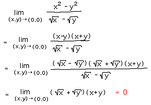
For example, find lim(x,y)→(0,0) (x2-y2)/(√x-√y) via repeatedly factoring differences of squares:
Limits that Don’t Exist
If in, say, a 2-path test, an expression turns out to 0/0 when you plug in the value being approached, does that mean the limit doesn’t exist?
No, the purpose of a limit is often to show that a function approaches a well-defined value as its arguments get closer and closer to a point where the function itself is undefined.
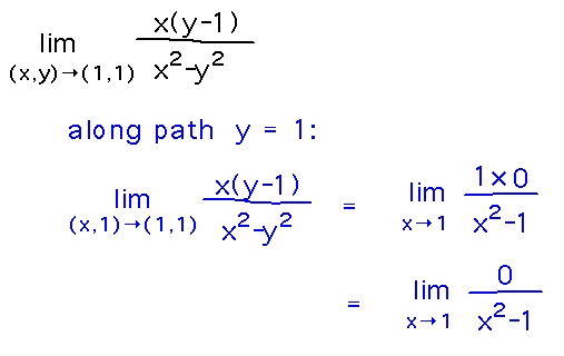
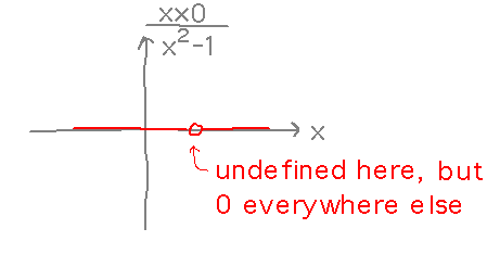
For example, along the y=1 path in the solution to problem 3 in the sample exam questions the expression inside the limit becomes 0/0 when x = 1, but at every other point of the form (x,1) the expression’s value is 0, so the limit is 0:
It’s maybe easier to see this if you plot the value of the expression as x approaches 1, while holding y constant at 1. The plot is a constant line at 0, even though the expression becomes undefined at 0 -- but no matter how close to 0 you get, as long you aren’t at 0, the expression’s value is still 0:
Level Curves
How do you calculate level curves?
Mostly, it’s much less exciting than it seems it should be: a level curve is simply a set of points or an equation that correspond to some function having a constant value.
For example, the level curve (or surface in this case) where the function f(x,y,z) = xy + cosz has constant value 1 is just described by setting the function equal to the constant: xy + cosz = 1.
You might be able to do things like find points on the level curve given values for some of the variables, but basically calculations with level curves are straightforward.
Level curves are, however, a concept that’s important in a lot of places. For example gradients are normal to level curves/surfaces, that in turn is central to the derivation of Lagrange multipliers as a way to solve optimization problems, etc.
Next
After the exam: Introduction to integration of multivariable functions. Read section 5.1.