Misc
Colloquium
Friday, February 16, 2:30. Newton 203.
“From Differential Equations to Difference Equations and Everything Else in Between.”
Differential equations define a continuous function in terms of its derivative(s); difference equations define a discrete function in terms of its difference(s).

Billy Jackson, SUNY Geneseo.
Extra credit for going and writing a short reaction.
Questions?
Integration with muPad
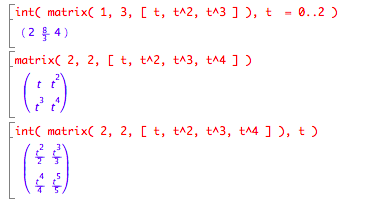
Vector valued functions that you integrate with muPad need to be defined as matrices of functions, nominally n-row-by-1-column.
Define matrices with the function matrix( rows, columns, [ components ] ) where rows is the number of rows, columns is the number of columns, and components is a comma-separated list of components.
Then the int function computes integrals, either definite or indefinite depending on whether you attach a range of values to the integration variable.


muPad will actually integrate any matrix of functions.
Arc Length of Space Curves
Theory
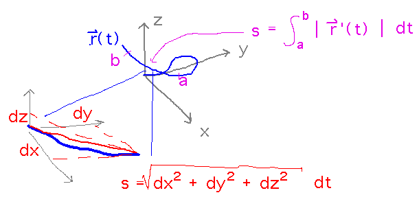
What’s the justification for the arc length formula?
It comes from approximating very short segments of the curve as straight lines and applying the distance formula, in a Riemann sum.
Example
Find the arc length of r(t) = 〈 sin 3t, cos 3t, 1 〉 from t = 0 to 2.
Start by finding the derivative of r:

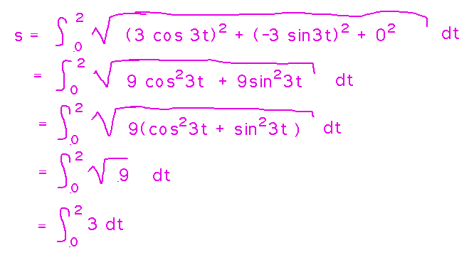
Then evaluate the arc length integral, taking advantage of a trigonometric identity to simplify it:
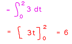
And finally evaluate the integral:
Arc Length Parameterization
Consider r(t) = 〈 t2, t2, t2 〉.
This function defines a straight line, i.e., the quadratic terms don’t affect the shape of the curve.
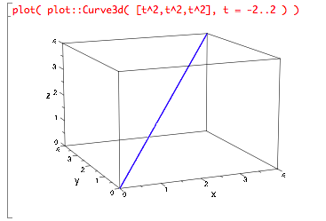
What they do affect is how “fast” you move along the curve at different t values. The value of t isn’t a guide to how far along the curve you have moved.
Some times you want to parameterize a curve in such a way that the parameter value tells you how far you’ve moved, e.g., “if t is now twice what it was before, I must be twice as far along the curve as before.” The arc length parameterization does this.
The strategy for finding a parameter that corresponds to distance:
- Find a function s(t) that gives you distance along curve in terms of t.
- If s(t) can be inverted, you can get an expression, t(s), for t in terms of distance.
- Plug that expression into r( t(s) ) to get position in terms of distance.
Here’s how that works for the function above. We’ll use the basic arc length definite integral, but with the upper bound on the integration being t and the lower bound being an arbitrary starting t value -- let’s use 0, though it could be anything. Then rename the variable inside the integrand to avoid confusion with t as the upper bound. The overall result is a function of t that integrates arc length from 0 to t, i.e., finds the length of r from parameter value 0 to parameter value t, which is exactly what we wanted.
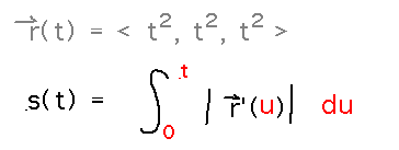
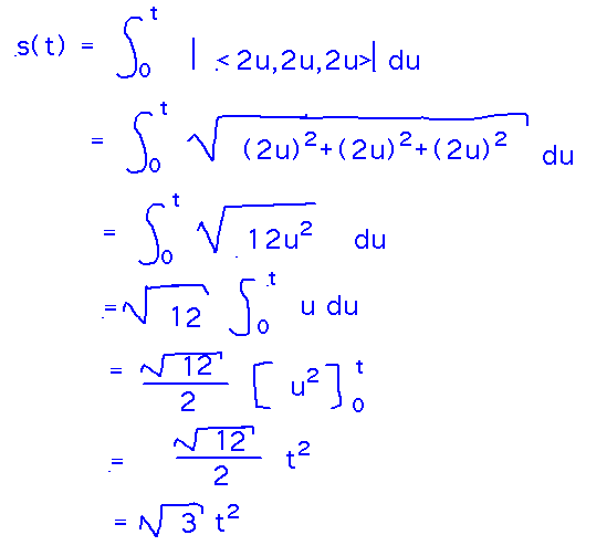
To use this on r(t) = 〈 t2, t2, t2 〉we need r’(t) =〈 2t, 2t, 2t 〉, or〈 2u, 2u, 2u 〉after renaming the parameter. Now plug that into the arc length integral and integrate:
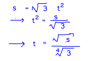
Now we have distance (s) as a function of t. To invert this and get t as a function of distance, rewrite to “solve” for t:
Finally, replace t in the original definition of r with the expression for t in terms of s to get the arc length parameterization of the curve:

Key Points
The arc length formula comes from the distance formula.
Using the formula to find arc length.
The arc length parameterization lets you express positions on a curve in terms of distance along that curve from some starting point.
Next
Curvature.
Read “Curvature” and “The Normal and Binormal Vectors” in section 3.3.