SUNY Geneseo Department of Mathematics

Green’s Theorem for Flux Integrals

Thursday, December 6

Math 223 01
Fall 2018
Prof. Doug Baldwin

Misc

Final

Friday, December 14, 8:00 AM

Comprehensive, but with emphasis on material since last hour exam (e.g., multiple integrals, line integrals, vector fields, Green’s Theorem, etc.)

Designed for 2 hours, you’ll have 3 1/3.

Rules and format otherwise similar to hour exams, especially open-references and calculator/computer rules.

I’ll put some sample questions on Canvas.

I’ll bring donuts and cider.

Review Session

11:30 - 12:30, Fraser 202A (our usual classroom), on study day.

SOFIs

5 responses. Thank you, but...

... please do submit more, they’re helpful to me.

Questions?

Green’s Theorem, Flux Form

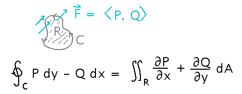
“Flux Form of Green’s Theorem” from section 6.4.

Yesterday we saw that flux line integrals (which are really just any 2D vector line integral with components interpreted right) meeting the requirements of Green’s Theorem can be expressed as double integrals:

Flux line integral around region equals a double integral over region

Example

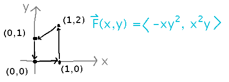
Use this idea to find the flux of F(x,y) = 〈 -xy², x²y 〉across the counterclockwise trapezoid with vertices (0,0), (1,0), (1,2), (0,1).

Trapezoid and vector field

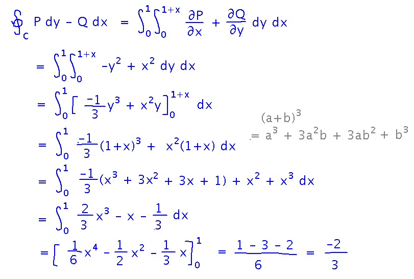
Since this is the same trapezoid we’ve used in earlier problems, the bounds for the double integral are still x ranging from 0 to 1 and y from 0 to 1 + x. Beyond that, put the Green’s Theorem flux formula inside the integrals and evaluate:

Integrate dP/dx + dQ/dy over region to find flux

Key Point

Flux via Green’s Theorem.

Source-Free Fields and Stream Functions

“Source-free” vector fields are analogous to conservative fields, but for flux. In other words, in a source-free field…

Flux line integrals along a curve from point P₁ to point P₂ can be evaluated simply by evaluating a “stream function” (analogous to a potential function) at P₂ and P₁ and finding the difference,
...and so flux line integrals around closed curves are always 0.

The term “source-free” suggests that the vectors don’t seem to originate at any particular point(s):

Vectors from a source pass through a curve, vectors without source circle along it

The components of a source-free vector field are related to the derivatives of the stream function, g, but in a different order than the components of a conservative field:

Vector field consists of dg/dy and -dg/dx

Example: determine whether F(x,y) = 〈 -y, x 〉 is source-free, and if so find a stream function. As with conservative fields, finding a stream function both shows that the field is source-free and (obviously) provides the stream function. So let’s try doing that. You can use the same strategy you used to find potential functions, namely integrate a component of F with respect to the appropriate variable to get an initial estimate, differentiate it with respect to another variable and compare to the corresponding component of F, etc. In this case, let’s start with the first component, -y:

Integrate -y to get -y^2/2 + h(x) as stream function

Now see what it would take for the negative of the derivative of g(x,y) with respect to x to equal the second component of F:

Derivative of stream function is derivative of h, which must equal -x, so h equals -x^2/2 + C

Now we have the complete stream function:

Stream function is -y^2/2 - x^2/2 + C

Key Points

An interesting analog of conservative fields.

You got some practice generalizing earlier ideas.

Green’s Theorem on more general regions: can any of the fine print that limits uses of Green’s Theorem be relaxed?

Read “Green’s Theorem on General Regions” in section 6.4.

Next Lecture