The Fundamental Theorem of Caculus, Part 1

Return to Course Outline

Previous Lecture

Questions?

How to do summations in Mathematica (actually asked at end of class):

The key function is Sum.

Here’s a demonstration of Sum with both numeric and variable upper bounds.

The Fundamental Theorem of Calculus, Part 1

First part of section 5.3.

Examples

Find the derivative...

This is a classic example of the Fundamental Theorem: the derivative of the integral is just the integrand, with x substituted for the variable of integration.

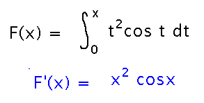
Another example, solved the same way:

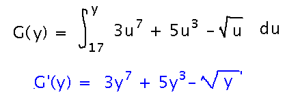
Notice that the lower bound of the integral doesn’t matter. This is because if you think about the integral as an area, and its derivative as how it’s changing with x, the amount of change depends only on what’s happening at the upper, “x,” end of the interval:

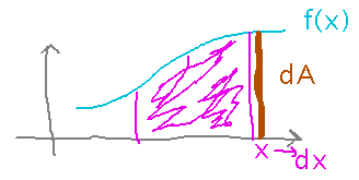
And in fact, the change in area depends on the value of f(x), not on its derivative or antiderivative. This is why the fundamental theorem doesn’t require you to change f in any way except to plug in x.

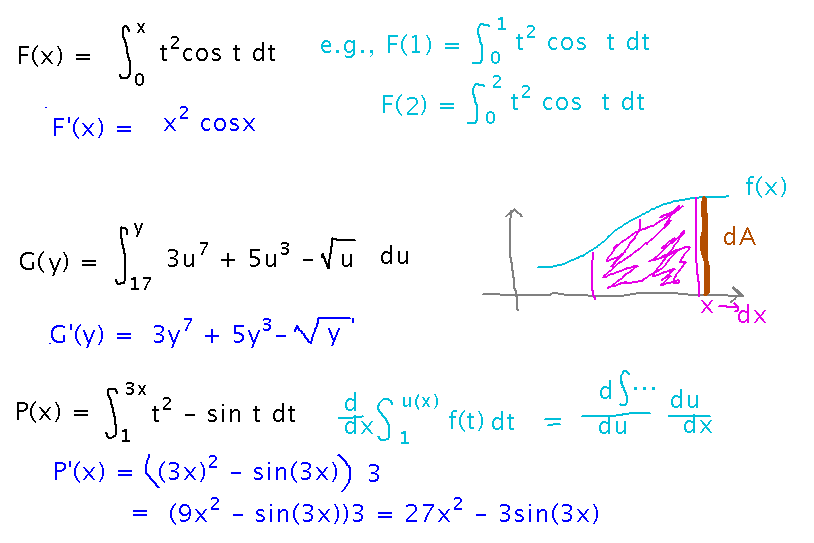
One final example:

Here the upper bound on the integral is a function of x. Blindly applying the fundamental theorem gives you the derivative with respect to that function, but to get the derivative with respect to x you need to use the chain rule on the upper bound:

Here are the above examples as the whole collection looked at the end our discussion of them:

Probability

A place where functions that are integrals up to some variable bound really do play a role.

“Discrete probability” is the sort you’re probably used to: for example, if I flip a coin, there are 2 possible outcomes, and so the probability of any one of them is 1/2.

But consider the following scenario: it takes me about half an hour to drive home from work. If I’m expecting a phone call, Murphy’s Law (“if anything can go wrong, it will”) says it will arrive while I’m driving, but there’s no particular reason to think it will arrive at any particular time. So intuitively, it seems that the probability of the call arriving t minutes after I start driving is 0 for t < 0 (i.e., before I start), 0 for t > 30 (after I finish), and some non-0 amount in between (technically the thing this intuition describes is a “probability density function,” which is like but not exactly the same as probability, for reasons seen below):

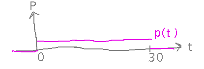
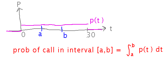
Now if I want to know what the probability of the phone call arriving at any particular time is, there are an infinite number of possibilities: 15 minutes 3.01852... seconds, 18 minutes 53.9735... seconds, etc. So the probability of the phone call arriving at exactly any one of them is 0 (which is why the pink line in the graph above isn’t strictly a graph of probability) — the question “what is the probability of the call arriving at exactly such-and-such a time” doesn’t really make sense to ask at all. Instead, you ask what’s the probability of the call arriving in such-and-such a range of times, e.g., between t=a and t=b? In that case, the probability is considered to be an integral (think of it as a sum of the infinitely many infinitely small probabilities of the call arriving at each time in the interval):

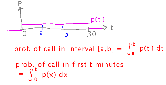
Now I can ask a related question, namely “what is the probability of the call arriving in the first t minutes of my drive,” and I get an integral with t as its upper bound:

Here’s how the above pictures looked as a whole when we finished talking about probability in class:

Key Points

Fundamental theorem (part 1), informally: derivatives get rid of integrals

Applying that idea, including using the chain rule if needed.

Next

The Fundamental Theorem, Part 2.

Read the rest of section 5.3.

Next Lecture