Misc
No SI session today, SI starts up again after break at the usual times (WF 3:00 - 4:30).
Questions?
What does the first problem on the new problem set (the speeding car) look like visually?
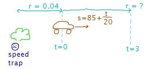
The point is to figure out how far past the speed trap the car is by the time the police officer realizes what they’re seeing. Note that this is an initial value problem.
Rates of Change in Triangles
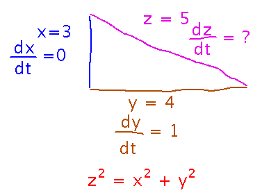
From yesterday, can the rate of change in the hypotenuse of a right triangle be calculated as the sum of the squares of the rates of change of the sides?
Unfortunately not. If you doubt some mathematical claim, a common way to disprove it is to find a “counterexample,” i.e., an example in which the claim doesn’t hold. All things being equal, simple counterexamples are better than complex ones, so here’s a fairly simple counterexample for this rate of change claim:
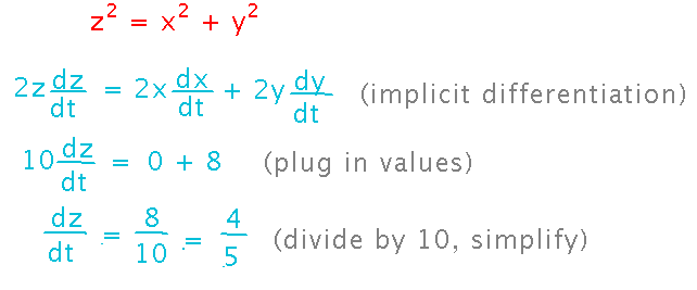
The actual rate of change in the hypotenuse can be found using implicit differentiation:
On the other hand, applying the Pythagorean theorem to the derivatives gives a different value:
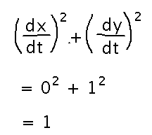
(Which gives dz/dt = 1, since the square root of 1 is 1)
Linear Approximation
Section 4.2
Estimation
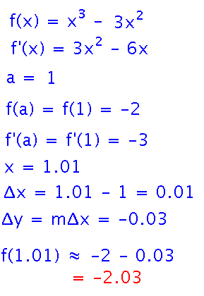
Use linear approximation to estimate the value of f(1.01) if f(x) = x3 - 3x2 and knowing f(1) = -2.
There’s an equation for this in the reading, which starts with the slope of the tangent to the curve:
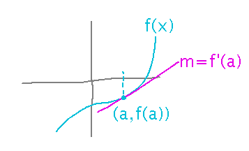
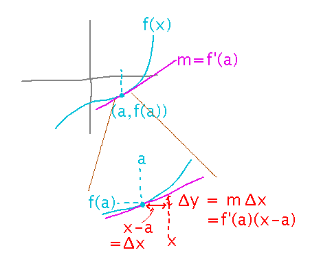
The idea is that close to x = a, the tangent is a reasonable approximation to the curve, and one that’s easy to evaluate: since slope is change in y over change in x, multiply the tangent’s slope (i.e., f’(a)) by the change in x (i.e., x - a) to get a change in y, and add that change to f(a):
Applying this to the specific example gives...
Notice that there is a gap between the straight line approximation to f(x) and the actual curve, i.e., the linear approximation isn’t exact. In principle, we could reduce the gap by also taking into account how fast the slope of f’s derivative increases or decreases, i.e., including f′′(x). And we could do better still by also including f′′′(x), and so forth. In the limit, as we include an infinite number of derivatives, we get something exactly equal to f. This is the basis for the so-called “series form” of a function, one of the major topics in calculus 2 (you may have heard hints of it under names such as “Taylor series”).
Linear Approximation and Differentials
In talking about slopes of lines, we talk about slope being a change in y over a change in x, i.e., Δy/Δx. The dy/dx notation for derivatives is motivated by a similar view of slope, i.e., dy represents an infinitesimally small change in y corresponding to dx, an infinitesimally small change in x. From this point of view it makes sense to think of the “Δy = f′(a) (x-a),” aka “Δy = f′(a) Δx,” part of linear approximation as multiplication and cancellation of parts of a derivative:
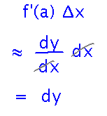
When dy and dx are separated in this way they are called “differentials,” and conceptually represent very small changes in y or x. Much of calculus can be understood as manipulation of differentials (although understanding it in terms of limits is more rigorous and connects better to other parts of math).
Next
Finding minima and maxima.
Read section 3.3