Area Between Curves, Part 2

Return to Course Outline

Previous Lecture

Anything You Want to Talk About?

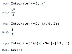
How to do integration in Mathematica. The basic function is Integrate, which takes a function to integrate as its first argument, and either the variable in that function (for an indefinite integral) or the variable and the bounds on its value (for a definite integral) as its second argument. For example...

You can download these examples as a Mathematica notebook if you want to explore them further.

Also see the November 23 class notes for a slightly longer explanation and more examples.

Area between Curves

Some of the more complicated problems from the area between curves discussion, based on “Area of a Region between Two Curves” and “Areas of Compound Regions” in section 6.1 of our textbook.

Curves that Cross

Find the area between the curves y = x³ and y = x² over the interval 0 ≤ x ≤ 2.

Looking at a graph of these two functions shows that they cross at x = 1:

There’s therefore no one function that is bigger than the other over the whole interval. You therefore have to split the region in which you’re finding the area between the curves into 2 regions, one in which x³ is bigger, and the other in which x² is, integrate over each region, and then add the results:

Having set the integral up, we then used it to get more practice with integration in Mathematica:

The general strategy for dealing with curves that cross each other is:

1. Find where the curves cross
2. Integrate f(x) - g(x) or g(x) - f(x) separately over each interval between crossings; which difference you integrate over a particular interval depends on which of f(x) and g(x) is larger over that interval
3. Add the results.

Alternatively, you can think of this as integrating the absolute value of the difference between the functions.

The “Kite”

What is the area inside this shape, bounded by the graphs of (x+1)², -2(x+1)², (x-1)², and -2(x-1)²?

There are a couple of interesting observations on this problem in the Canvas discussion, worth presenting in more detail.

The first is that the figure is symmetrical left to right, so you can find the area of just one side (say, the left side) and double it to get the area of the whole figure. Set up the integral for that area using the absolute value of (x+1)² - -2(x+1)² as a reminder that the curves might cross:

Having set up that reminder, now we have to act on it, i.e., figure out whether the curves really do cross and if so where. It turns out they don’t, and in fact the two functions can be combined to form a slightly simpler integral:

Now, although we could FOIL out the (x+1)² term, it’s easier to get rid of it by doing a substitution, which let’s us finish the integral:

This demonstrates how you can find areas of regions bounded by multiple curves, or by functions defined piecewise. The general strategy is very similar to that for curves that might cross:

1. Identify intervals bounded above and below by each pair of functions (may involve solving equations)
2. Break the integration up according to those intervals
3. Figure out which function is larger and which smaller in each interval.
4. Integrate differences
5. Add up results.

An Explicitly Piecewise Function

Suppose g(x) = 3 if x ≤ 0 and g(x) = x if x > 0. What’s the area of the region between g(x) and f(x) = x² - 1 over the interval -2 ≤ x ≤ 1?

This time g(x) is greater than f(x) over the entire interval, but we still have the break the integral into pieces corresponding to the pieces of g(x). (You can similarly break up an integral to integrate a single piecewise function, or one that has a finite number of discontinuities.)

Once again, we can have Mathematica evaluate the integrals:

Question: since g(x) is not actually equal to x at 0, don’t you have to somehow exclude 0 from the second integral? It turns out you don’t: the value of the integral is what you get as the lower bound gets closer and closer to 0, i.e.,

This limit can be evaluated just by substituting 0 for a, which is exactly what you’d do if you evaluated the original integral with a lower bound of 0.

Next

You can also use integrals to find volumes. One way is to think of a volume as a stack of thin slices, and to then calculate a Riemann sum of the volumes of all the slices.

Please read “Volume and the Slicing Method” in section 6.2 by class time Wednesday.

Also work on and contribute to the examples in this discussion of volume by slices.

Next Lecture