Absolute Extreme Values on an Interval

Return to Course Outline

Previous Lecture

Anything You Want to Talk About?

(No.)

Misc

Problem Set 7

...is now available.

It focuses on related rates, and to a slightly smaller extent on extreme values.

Work on it this week, aiming to grade late this week or early next.

SI

The next session is scheduled for Tuesday 4:00 - 5:30. Emiliana will confirm with an announcement and link tomorrow.

Extreme Values and Closed Intervals

From “Locating Absolute Extrema” in section 4.3 of the textbook and this discussion of extreme values on closed intervals.

Key Idea

Endpoints matter! They aren’t necessarily critical points (i.e., points where derivatives are 0 or undefined), but they are nonetheless points where minimums or maximums might occur.

A process for finding extreme values on closed intervals:

1. Find critical points as usual, and calculate the function’s value at them
2. Calculate the function’s values at the endpoints of the interval
3. The absolute minimum/maximum on the interval is the minimum/maximum of the values from the critical points and the endpoints.

Example

(From the discussion.)

Imagine a fictitious and somewhat tongue-in-cheek study of math professors, which finds that their production of good ideas varies with time of day, according to the formula

where t is hours since midnight, and P(t) is the number of good ideas the professor produces at time t. At what time between 8:00 AM (t = 8) and 5:00 PM (t = 17) should you approach a math professor in order to get the most good ideas from them? When between those same times should you expect the professor to have the fewest good ideas?

Start by finding critical points, so take the derivative of the productivity function and start solving for t values that make it 0. At first, that’s just calculus and standard algebra, despite the trigonometric functions.

Now we need to use some special knowledge of trigonometry, namely angles at which sine and cosine are equal. There are 2 such angles between 0 and 2π:

Knowing this, finish solving for places where dP/dt is 0:

There are no places where the derivative is undefined, so these two values are the only critical points. One of them, t = 3, is outside the interval we’re interested in, and so can be discarded now. We need to calculate productivity at the other critical point (t = 15), and at the endpoints of the interval (t = 8 and t = 17) and see which produces the highest and lowest productivity values:

So apparently it’s best to ask a math professor (or at least one of these fictitious ones) questions at 8 in the morning, and worst to do it at 3 in the afternoon.

Another Example

The power that a hypothetical new car needs in order to maintain a steady speed of s miles per hour is given by

(This formula is fictitious, but based on 2 pieces of reality: at high speeds, a car’s power consumption is dominated by friction, which increases as the cube of speed, and at lower speeds it generally decreases until speed reaches some engineering design optimum that is often in the 50 - 60 mph range.)

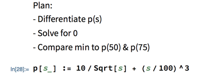
This problem is a good one to use Mathematica on, so use it to do a lot of the numeric and symbolic work in the following (but don’t just use the Minimize function that Mathematica turns out to have):

If you’re driving this car on the highway, and willing to drive at any speed between 50 and 75 mph, what speed should you pick to minimize power consumption (and thus maximize fuel economy)?

We started by writing down an outline of the plan as a comment (use “Style -> Text” in Mathematica’s “Format” menu to tell it that a cell is a comment instead of a command to execute), then we defined our power function p(s), so that we can use it later in the problem (last Friday’s class notes say more about defining your own functions in Mathematica):

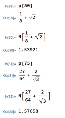
Having defined p(s), we tried it out, and while doing so calculated p(50) and p(75), the values at the endpoints of the interval. Mathematica initially gave symbolic answers for these values, but we converted them to decimal numbers using the “Numerical Value” button that appears below the output; you can do the same thing manually with Mathematica’s N (for “numeric value”) function:

Finally, we had Mathematica differentiate p(s) and solve for places where it’s 0. Notice that Mathematica has a Solve function built in that solves an equation for the value(s) of one or more of its variables. The general form is

Solve[ equation, variable ]

where equation is the equation to solve and variable is the name of the variable to solve for. Be careful that the “=” sign in an equation has to be written as two equal signs, ==, in Mathematica:

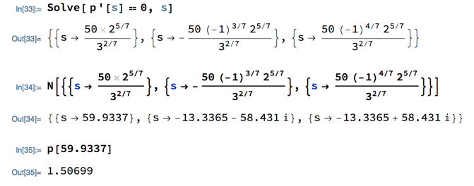
Notice that Mathematica found 3 places where dp/dx is 0, but 2 of them turn out to be complex when looked at numerically, so only the solution around 59.9 is relevant to our problem. Comparing the p function at the endpoints of the interval to p(59.9337) shows that 59.9337 mph is the speed that is most efficient to maintain, i.e., requires the least power.

You can download a copy of the Mathematica notebook with the above calculations from Canvas if you want to experiment with them for yourself.

Next

The Mean Value Theorem: a result that in some ways seems innocuous (once you understand it at all), but turns out to be important in connecting derivatives to the general behavior of functions, to antiderivatives, etc.

Please read section 4.4 in the textbook by class time Wednesday.

Please also contribute to this discussion of the Mean Value Theorem by class time Wednesday.

Next Lecture