Extreme Value Examples, Part 2

Return to Course Outline

Previous Lecture

Anything You Want to Talk About?

(No.)

SI

Sunday 6:00 - 7:30

Then Tuesday 4:00 - 5:30

Extreme Values

From “Absolute Extrema” and “Local Extrema and Critical Points” in section 4.3 of our textbook, and this extreme values discussion.

Geometry Example

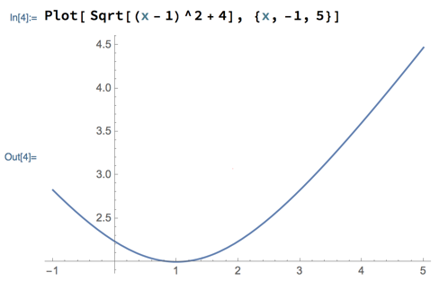
Intuitively, the point on the x axis that is closest to point (1,2) is (1,0), the point directly below (1,2). Show that this intuition is right.

Start by phrasing this question as an extreme value problem. In particular, think about the distance from point (1,2) to any point on the x axis, i.e., point (x,0). You can find this distance via the Pythagorean Theorem:

Now you can find the x value that minimizes this distance, and see if that value really is 1.

As usual, start by finding the derivative of L:

Then find values of x that make the derivative 0:

Since the goal was to see if x = 1 minimizes distance to the x axis we’re done here, although it might also be interesting to plug x = 1 into the formula for L and verify that L(1) = 2 (which we already know is the vertical distance from point (1,2) to the axis).

While solving this problem, the question came up of what the graph of L looks like, and what to expect of the derivative of L (i.e., the slopes of that graph). Here’s L plotted with Mathematica:

Some Technicalities

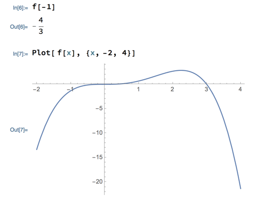
Where are the local minima and maxima (if any) of f(x) = x³ - x⁴/3?

Differentiating f and setting the derivative to 0 yields…

Figuring out which critical points correspond to minimums and which to maximums could involve evaluating the function at various places, but if we’re going to do much of that there’s an easier way: have Mathematica do it!

When you’re working with a function of your own in Mathematica, it’s convenient to be able to give it a name and use it like you would other functions in Mathematica. You can in fact do this. To define your own function, enter a command that consists of the name you want the function to have, followed by its argument suffixed with an underscore (“_”) inside square brackets, followed by “:=”, and finally followed by the expression the function evaluates. For example…

Once you define the function, you can use it like any built-in function. For example, you can ask for its value at any x value you like, you can plot it (a good way to see its value at lots of places all at once), etc.

You can download a Mathematica notebook that demonstrates these commands, and in which you can try variations on them, from Canvas

For the example function, the plot suggests strongly that there’s a maximum at x = 9/4, but what about x = 0? Visually, it could be a minimum or maximum that just involves too small a peak or trough to see in this plot, or it could be neither. It can’t be a maximum, because if it were there’d have to be a minimum between it and the maximum at 9/4 (as long as f is continuous, which it is):

But we don’t have another critical point between x = 0 and x = 9/4. Similarly, there can’t be a minimum at x = 0, because there would need to be a maximum between x = 0 and the clearly smaller values corresponding to negative x values. So x = 0 must be a critical point that doesn’t correspond to an extreme value at all.

There are two morals from this example:

1. Not all critical points correspond to extreme values.
2. You can use rigorous mathematical analyses (like finding critical points, along with the logic of how they alternate, in this example) to back up less rigorous intuitions (like estimating the function’s behavior from a plot in this example) to produce perfectly rigorous results (like the conclusion that there is neither a minimum nor maximum at x = 0 in this example).

Next

Extreme values on closed intervals, i.e., intervals with well-defined endpoints.

Read “Locating Absolute Extrema” in section 4.3 of the textbook by class time Monday.

Also participate in this discussion of absolute extreme values on closed intervals by class time Monday.

Next Lecture