Extreme Value Examples

Return to Course Outline

Previous Lecture

Anything You Want to Talk About?

(No.)

Extreme Values

From “Absolute Extrema” and “Local Extrema and Critical Points” in section 4.3 of our textbook, and this extreme values discussion.

Radio Example

Picking up the example of how radios tune in certain frequencies and tune out others (so, e.g., your cell phone gets people who want to talk to you, but not the TV or radio station down the street) via circuits whose resistance to electrical signals varies with the frequency of those signals. Wednesday I introduced a simple model of such a circuit in which resistance, R, might be equal to f + 1/f where f is frequency. Wednesday we also started to find out where such a circuit has its minimum resistance; we were following the plan for solving extreme value problems listed in Wednesday’s notes (differentiate the function in question, find values of x that make the derivative 0, find places where the derivative is undefined, and finally plug the x values from the previous 2 steps into the function). We had already found the derivative, so results so far looked like…

To finish solving this problem, we first need to find places where the derivative is 0:

Notice that one of the solutions, f = -1, is mathematically possible but not physically possible (radio waves can’t have a negative frequency), so we discarded it.

Next we should identify any places where the derivative is undefined, which happens at f = 0.

Finally, the critical points, i.e., f values where the derivative is either 0 or undefined, are all candidates for places where the minimum R occurs. So plug each of those values into the equation for R, and see which produces the smallest value.

Notice that when f = 0, R is undefined, but to get a sense for the way in which it’s undefined, we looked at the limit of R as f approaches 0 (from the right, since negative frequencies don’t make sense in this problem).

Mathematica

With problems such as extreme values, we get to a kind of math where tools like Mathematica are valuable. So far we’ve used Mathematica as a source of single, specific, functions to use in specific contexts; now we can approach it more as a toolbox from which to pick and choose functions that illuminate a problem in whatever way we find interesting.

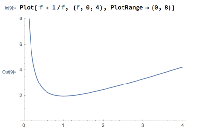
In the radio example (and many extreme value problems), it’s often interesting to plot the function near its critical points to see how it reaches maximum or minimum values. So I did that with the resistance function.

In doing this though, we discovered that Mathematica, left to its own devices, only plots from y = 2 to about y = 6 (the smallest and largest y values actually needed by the plot). Not having the y axis extend down to 0 is unintuitive, so we wanted to control the range of values on the y axis ourselves. To see if this is possible, we used Mathematica’s “Help” menu to look at documentation on the Plot function, and discovered the PlotRange option. Plotting the resistance with this option looks like this:

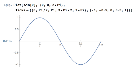
Then someone asked if it’s possible to control where Mathematica places tick marks along the axes, e.g., for plotting trigonometric functions, can you put tick marks at π/2, π, etc. rather than at integer positions? I didn’t have a quick answer to this question, but looked into it after class and discovered the Ticks option for Plot. This option needs 2 lists of tick mark locations, one for the x axis and one for the y; each list is enclosed in curly braces, with the pair of lists enclosed in another set of braces. For example, here’s how to plot a sine wave with tick marks on the x axis at multiples of π/2 and tick marks on the y axis at multiples of 0.5:

Geometry Examples

Intuitively, the point on the x axis that is closest to point (1,2) is (1,0), the point directly below (1,2). Show that this intuition is right.

Start by phrasing this question as an extreme value problem. In particular, think about the distance from point (1,2) to any point on the x axis, i.e., point (x,0). You can find this distance via the Pythagorean Theorem:

Now you can find the x value that minimizes this distance, and see if that value really is 1.

We didn’t have time to do this in class today, but try to keep working on it in the extreme values discussion, and we’ll finish it tomorrow.

Next

The geometry example via the discussion, and a few more examples. No new reading.

Then extreme values on closed intervals, i.e., intervals with well-defined endpoints.

Read “Locating Absolute Extrema” in section 4.3 of the textbook by class time Monday.

Also participate in this discussion of absolute extreme values on closed intervals by class time Monday.

Next Lecture