Anything You Want to Talk About?
Setting up video chat for your individual meetings with me: you can add a Zoom or Google meetings link to your meeting in Google calendar, or you can use my office hours Google meeting (https://meet.google.com/boo-wyaj-hcr). Or talk with me about setting something else up.
Misc
SI
Introduction from Emiliana.
The SI program is a really helpful one, take advantage of it.
Please fill out the Doodle poll about possible times for SI sessions by Monday. Sessions will meet twice a week, by Zoom, for 1 1/2 hours per session. They will probably start next Tuesday or Wednesday.
Canvas Organization
A couple of posts in the policies and practices discussion suggested different ways of delivering class information, e.g., videos showing examples of problem-solving techniques, video overviews of the course by week or unit.
Sadly, good-quality videos are probably too time-consuming to produce for every class, but I could certainly organize information differently in Canvas (e.g., textual or diagrammatic overviews by week or topic, thematic rather than chronological summaries, etc.), and maybe do videos for a few particularly important topics.
More ideas, or support vs disapproval for existing ones, welcome. Share them via email or in an individual meeting if you don’t want to make them public, or go back to the “ideas you have” part of the policies and practices discussion (which is public).
Intuition for Limits
The “Intuitive Definition of a Limit” and “The Existence of a Limit” subsections in section 2.2.
Key idea: For a function f(x) and a constant c, the limit of f(x) as x approaches c (written limx → c f(x)) is the value that f(x) heads towards as x gets closer and closer to c, both from above c and from below.
Spreadsheet Example
Estimating limx → 1 (x3 - 3x2 + 3x - 3) / (x-1) via a table and plot. What are you looking for in the spreadsheet to estimate that limit?
Whether the numbers in the “f(x)” column converge towards a common value as the corresponding numbers in the “x” column approach 1 from both sides. In this case, they do, f(x) seems to converge towards (and indeed reach, at least to within the accuracy of the spreadsheet) 0.
The graph is also helpful, you can see visually that the line of the graph drops towards 0 from both sides as x gets closer to 1.
Question: how do you know what values of x to use? There’s no hard-and-fast rule, but the general goal is to see what the trend in f(x) values is as x gets close to 1, and to do so from both sides of 1. So a good start is to probably start with 2 values slightly smaller than 1, and 2 slightly larger, and see if the corresponding f(x) values do in fact seem to be heading towards some common place. Then add in more values as needed, until you feel you see a common limit from both sides (or see that there clearly won’t be).
Manual Example
The discussion claimed (correctly, but by using algebraic methods) that limt → -2 (t2-4) / (t+2) = -4. Let’s build a table to see if this claim makes intuitive sense.
We started with t = -2.0001 and t = -1.9999. Both seemed to yield g(t) near -4, but since these values are on opposite sides of -2, they don’t show what any trend in g(t) is as t approaches -2. So we added two more values, namely -2.1 and -1.9. Now we have two values below -2, and two above, and both pairs suggest that g(t) approaches and passes through -4 as t gets closer to -2. (But in reality g(t) doesn’t “pass through” -4, because it is undefined at t = -2.)
| t | g(t) |
|---|---|
| -2.1 | -4.1 |
| -2.0001 | -4.0001 |
| -1.9999 | -3.9999 |
| -1.9 | -3.9 |
Absolute Value Example
There was some debate in the discussion (good!) about limy → 0 |y| / y. Most recently it seems to be tending towards the limit not existing (which is correct). Can we come up with tables of values and/or graphs that demonstrate that?
A graph is probably clearest: as y approaches 0 from below (i.e., y is negative), |y|/y equals -1. So the graph clearly seems to be approaching (and in fact is at) -1. But on the other hand, as y approaches 0 from above (y is positive), |y|/y = 1, so the limit seems to be 1:
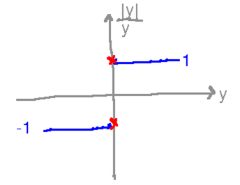
Since a limit is a single, unique, number that a function approaches, the limit does not exist in this case. There’s no single number the function approaches, since it “approaches” different values from the positive and negative sides.
Limits and Defined Values
Probably the most common use of limits is to find surrogates for the value of a function at a point where the function isn’t defined (as in all the examples above). But is this always necessary?
For example, does it make sense to talk about limx → 3 x2? Yes, the limit is what you get by plugging 3 in for x, i.e., 32 or 9. Such a limit is a perfectly valid thing to talk about and evaluate, although doing so seems like overkill for most practical purposes.
Problem Set
There is a problem set on the intuitive idea of a limit, which has been around in Canvas for a couple of days, but that I’m only “officially” assigning now.
You should be doing it during the next week.
If you have an individual meeting with me late next week, say Thursday or Friday, you could plan to grade the problem set in that meeting. If your individual meeting next week is earlier in the week, it might make more sense to grade in the following week’s meeting (especially if it’s also early in the week).
Two of the questions ask you to use Mathematica to plot functions. There is a nice “getting started” introduction to Mathematica in this video:
(It is a little weird that in the middle the video describes the general structure of all Mathematica commands via examples of functions that you would probably never use in the forms shown - they correspond to the standard arithmetic operations +, -, etc. But the message in that part that all Mathematica commands have a standard form is valuable.)
The video ends with an example of the Mathematica command for plotting functions, Plot. I’ll also make sure there are some examples of it in Wednesday’s class notes.
Next
We’re ready to move on to algebraic methods of finding limits. Read “Evaluating Limits with the Limit Laws,” “Limits of Polynomial and Rational Functions,” and “Additional Limit Evaluation Techniques” in section 2.3 of the textbook.
We also need to talk about plotting in Mathematica. Watch the video above.
And we might want to talk about tips on how to read mathematical material such as in the textbook.
My plans for this course have several days budgeted for algebraic ways of finding limits, so we have time to talk about any or all of these things as needed.
Watch for a new discussion soon to get the conversation started.
Reminder: the next class meeting is Wednesday, September 9 (Monday is a holiday); it is a Cohort C class.