Anything You Want to Talk About?
The problem set on intuitive understanding of limits: It got published earlier than I intended, I will officially assign it tomorrow.
Discussing it with me in an individual meeting: the idea is that you will work on it during the range of dates at its beginning (next week, basically). If you have an individual meeting with me late in that period (say, Thursday or Friday next week), it’s reasonable that you could be finished with it by then and discuss it. But if your individual meeting for next week is early in the week (say Tuesday or Wednesday), then it’s more reasonable to use that meeting for other things (e.g., let me know what is or isn’t working for you in the course, ask questions about the problem set or readings, etc.) and grade the problem set in the following individual meeting (presumably early in the week after next).
Calculus Preview
Section 2.1 in the textbook.
Speed from Position
The real-universe tornado scenario from the current discussion.
“Average rate of change” is a good way to solve this, but what exactly does that mean? Where is the “change” in the formula, where is the “average”?
Given a function whose graph goes through points

How do you make an average rate of change more accurately estimate the instantaneous speed of the tornado? Make the difference between x1 and x2 smaller.
What does this have to do with the reading? This is how the book works out a slope of a tangent line, i.e., a derivative, from the slopes of lines between nearby points on a function’s graph.
Position from Speed
The alternate-universe tornado scenario.
“Do average rate of change in reverse” is a good intuitive answer, but what do the details look like? One way to derive those details is to solve the average rate of change formula for the second y value in terms of rate of change (call average rate of change v, since in this problem it’s a speed or velocity).

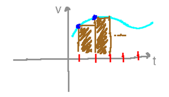
In terms of functions’s graphs, this is multiplying the value of a rate-of-change function by the length of an interval in x, and then adding it to an initial position. Doing that for one big interval won’t necessarily give a very accurate final position, but you can improve accuracy by doing the multiplication for a short interval, adding it to the initial position to get an estimated second position, then doing the multiplication over a second short interval and adding the product to this second position to get a third, and so forth.
Each of those products is also the area of a rectangle under the rate-of-change function’s graph:

But these areas of rectangles is just how the book defined an integral.
So here’s a very surprising result: areas under curves are somehow inverses of rates of change! In other words, to turn known rates of change into a function that would have those rates of change, you find the area under the rate-of-change curve. This is something called the Fundamental Theorem of Calculus, and is what ties derivatives and integrals together into a coherent subject (calculus).
Next
Both of the key calculus concepts, derivatives and integrals, involve limit processes, i.e., making some interval smaller and smaller and asking what happens to some formula involving that interval as its length gets closer and closer to 0. So in order to explore calculus, we need to start by understanding limits.
Tomorrow (Friday) through Wednesday, try to understand intuitively what a limit is.
Read the “Intuitive Definition of a Limit” and “The Existence of a Limit” subsections in section 2.2 of the textbook by class time Friday.
Do this discussion (or at least some of it) by class time Friday.