Rates of Change

Return to Course Outline

Previous Lecture

Misc

Colloquium

The first math department colloquium of the semester is this Wednesday (Sept. 25).

Sedar Ngoma (Geneseo)

“Rate of Convergence Resulting in a Finite Difference Approximation”

September 25, 2:30 - 3:30, Newton 201.

Up to 2 points problem set extra credit if you go and write me a paragraph on connections you make between the talk and your other interests, experiences, courses, etc. (Or any other reflections you have on the talk.)

SI Session

This evening, 6:00 - 7:30, Fraser 104.

Questions?

Taking derivatives in Mathematica? Be very careful that Mathematica always needs arguments to functions in square brackets, even if the function is a standard mathematical one. Thus, for example, Sqrt[t^2-t], not Sqrt(t^2-t).

Applications of Derivatives as Rates of Change

Section 3.4 in the textbook.

Key Ideas

The amount of change formula: f(x+h) = f(x) + h f’(x)

Derivative relationships, e.g., between position, velocity, and acceleration, also lead to antiderivative relationships that can be exploited in initial value problems.

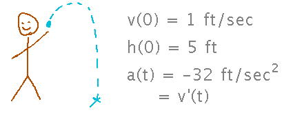
A Physics Example

Suppose I throw a ball into the air so that its initial (i.e., at time 0) velocity is 1 ft/sec (positive velocity is up), its initial position is 5 feet above the floor, and its acceleration is -32 ft/sec².

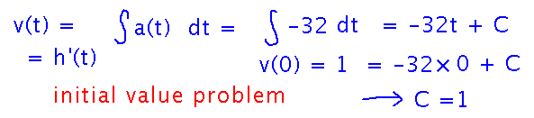
Find a formula for velocity as a function of time.

You know that velocity is the derivative of position, and acceleration the derivative of velocity, but those don’t help directly because you don’t have the position function to differentiate. But they do help indirectly, because they tell you that velocity is the antiderivative of acceleration, and position the antiderivative of velocity.

Furthermore, you can find the constant of integration in the antiderivative by setting it to make v(0) = 1, as specified in the problem description. This piece of information makes this an initial value problem.

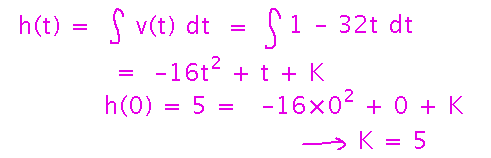
Find a formula for height as a function of time.

This goes very similarly to finding velocity, i.e., find the general antiderivative of velocity and then use the initial height to solve for the constant of integration:

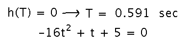
When does the ball hit the floor?

When h is 0. So solve the equation for h for the positive T that makes h(T) = 0:

A Business Example

If you’re in the widget (or any other manufacturing) business, the optimal number of widgets to manufacture is the number at which the marginal cost of making them just equals the marginal revenue from selling them.

Why? Because if marginal cost exceeds marginal revenue then you lose money by making 1 more widget, while if marginal revenue exceeds cost you can gain money by making 1 more. The place where these two considerations exactly balance each other is when marginal cost equals marginal revenue.

Next

Start working our way to derivatives of the trig functions.

But figuring out what their derivatives are requires some new understanding of limits, especially limits of trig functions, for which something called the squeeze theorem is helpful.

So read subsection “The Squeeze Theorem” in section 2.3 of the textbook.

Next Lecture