Misc
Math Olympiad (formally, the 13th University of Rochester Math Olympiad)
A college-level regional math competition
Saturday, February 9
Contact Prof. Towsley for more information or if interested in participating.
Questions?
Preview of Calculus
Section 2.1.
Instead of doing calculations for the following examples by hand, I did them in this spreadsheet: https://docs.google.com/spreadsheets/d/1WPPbGuZVDO6eLpfdfTyE-BCFTy6dTao3gh7UBKe9100/edit?usp=sharing
Rates of Change
Suppose you are Galileo with your ball-on-inclined-plane experiment, and thus now know that on a certain inclined plane, the ball rolls a total distance of t2 units in t time units:
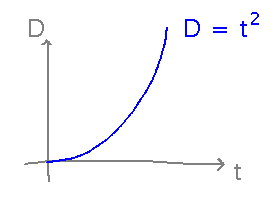
Estimate the ball’s instantaneous speed at t = 1.
What does the reading have to do with this? This is basically about secant lines, i.e., how lines between two points on the curve approximate the slope aka rate of change of the curve in between those points.
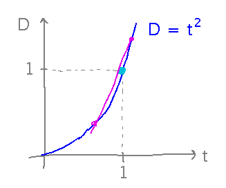
Notice that the formula for speed (distance traveled divided by elapsed time) is exactly the same as the formula for the slope of the secant line (change in D divided by change in t).
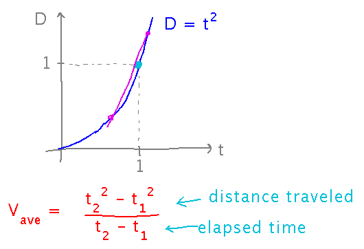
The spreadsheet has some estimates of speed around t = 1, for various different combinations of t value.
Notice that the smaller the difference between starting and ending t, the closer the calculated speed should be to the speed exactly at t = 1. For ultimate accuracy, make this change in t as small as possible.
Going the Other Way
Suppose you are the Galileo of some weird alternate universe, in which you were able to discover that the ball’s speed after t time units is t2 distance units per time unit. Estimate how far the ball travels in t time units.
What does this have to do with the reading? Distance covered at a given speed over a given time is the speed multiplied by the time. But on a speed-vs-time graph, those products are also the areas of certain rectangles on the graph. So finding distance from speed turns out to be the same calculation as the book’s estimation of area under a curve from the areas of many thin rectangles.
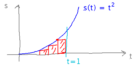
The spreadsheet has an example of this calculation, for 2 rectangles. Of course, the distance estimate would get more accurate as we used more but thinner rectangles.
Here’s a surprising discovery: the speed-from-distance and distance-from-speed calculations were opposites (technically, “inverses”) of each other. Speed from distance was basically a slope or rate-of-change calculation; distance-from-speed was basically an area calculation. Who would have though that area is the inverse of slope? This turns out to be a very important and useful result in calculus.
Next
In both the speed-from-distance and distance-from-speed examples above, the idea of what value some calculation reaches as something else approaches some limit was crucial to how accurate the estimates were. Let’s start to develop some more precise ways to work with that idea of limit values.
Read the introduction to section 2.2 of the textbook, and subsections
- Intuitive Definition of a Limit
- The Existence of a Limit
Starting Monday, please bring your laptop to class each day. I won’t have pre-planned activities with it every day, but it’s too likely that it will be spontaneously useful, if for no other reason than that you can pull up the Canvas notes, book, etc, on it.