Anything You Want to Talk About?
The recent announcement that all classes will be online-only after Thanksgiving: this will affect us only slightly. The basic structure of the course will continue the same as it is now, namely readings, online discussions, problem sets, and individual meetings with me. We won’t have face-to-face meetings to supplement the online discussions, and as a result I will probably take a more active role in the discussions. I will also keep posting summaries of the key ideas from discussions and readings, which is pretty much the role I see the daily class notes playing. I will try to keep up the current pace of roughly one topic every class day or so.
Misc
There’s an SI session Sunday, 6:00 - 7:30. Watch for announcements with a Zoom link.
Derivatives in Mathematica
The function for taking derivatives is D. Like all built-in Mathematica functions, the name starts with a capital letter, and arguments go in square brackets. The arguments are the expression to differentiate, and the name of the variable in that expression. For example…
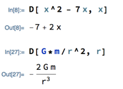
The second of these examples indicates why you need to tell Mathematica what the variable is: some expressions use letters to stand for things that aren’t variables, or at least aren’t the variable you’re interested in.
(You can download a Mathematica notebook with all of today’s examples from Canvas.)
Graphs and Derivatives
COVID-19 case information is often presented in two different ways: cumulative totals (i.e., the total number of cases in a country since the start of the pandemic) and daily new cases (the number of cases reported on a particular day, or often the average number of new cases over a short time period ending on a particular day). If you compare a cumulative graph with a daily new cases graph, you might understandably come to completely opposite conclusions. From the cumulative graph it looks like infections are rising; from the new cases graph it looks like infections are falling.
What’s going on?
The answer is that the new cases graph is the derivative of the cumulative cases graph. In other words, the number of new cases reported today is today’s change in the total number of cases since the start of the pandemic. Thus if the total number of cases is growing, but doing so more slowly than it did in the past, the daily cases graph (the derivative) will be dropping. Similarly, at times when the total number of cases is growing fast, the daily new cases will be high, whereas when the cumulative total is growing slowly, the daily new cases will be low.
Higher-Order Derivatives
In other words, derivatives of derivatives.
Try finding some second and higher order derivatives. You can do this by using the differentiation rules we know on the function, then on its derivative, then the derivative’s derivative, and so forth.

Notice that eventually the derivative became 0. This always happens eventually with polynomials. How many derivatives (i.e., first derivative, second derivative, third derivative, etc.) can you take of a degree-n polynomial (i.e., a function of the form f(x) = anxn + an-1xn-1 + … + a1x + a0 before the derivatives stop changing?
You can take n+1 derivatives: the first n progressively turn the xn term into x0 times some coefficient, i.e., a constant, and the (n+1)th derivative turns that constant into 0.
Why 0 and not 1? Conceptually, because the slope of a constant function is always 0; the power law for derivatives doesn’t apply when the exponent is 0. (See the proof of the power law in yesterday’s class notes for why the power law doesn’t apply to 0.)

You can also take higher-order derivatives in Mathematica, in either of two ways.
One interesting one is to use D on the result of another D operation:
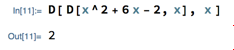
This example illustrates a general (well, mostly general; it didn’t work when we tried it with D and Plot) principle in Mathematica: you can compose operations together, i.e., apply one operation to the result of another.
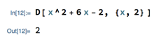
The second way is to use an option in the D function, whereby you can group the variable and the number of derivatives you want together in braces. For example:
Antiderivatives
Find a function whose derivative is 2x + 1.
You can informally reason this out by asking how the differentiation rules would produce the function in question, e.g., how would the power rule produce “2x,” how would it produce “1,” etc.

The resulting function is an “antiderivative,” and what we just did gives you an informal way to calculate them.
For a more formal approach to antiderivatives, we can work backwards from each differentiation rule to find a corresponding antiderivative rule (actually, we’ll see that this isn’t always possible, but for now we can do it). Here are some examples of antiderivative rules:

The antiderivative constant rule is interesting, because it implies you can always throw a constant onto the end of an antiderivative (and it can be any constant, there’s no specific value it has to be — that’s why it’s written as “C” above instead of an actual number). And in fact, it’s conventional to do that when finding antiderivatives. The example above is better written as

Next
Differentiation rules for products and quotients. (We will probably spread these rules over 2 class meetings, but that might take the form of simple uses in one class and more complicated ones in another, so I’d like to read about them and discuss them online as a group.)
Please read “The Product Rule” and “The Quotient Rule” in section 3.3 of the textbook by class time Monday.
Please also participate in this discussion by class time Monday.