SUNY Geneseo Department of Computer Science
CSci 120, Spring 2014
Prof. Doug Baldwin
Due Tuesday, March 4
Matlab can plot functions in 3 dimensions as well as in 2—in other words, it can plot functions of the form z = f(x,y), parametric lines in which three coordinates—x, y, and z—are functions of parameter t, etc.
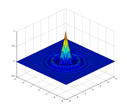
Two crucial Matlab functions for 3-dimensional plotting are the surf and mesh functions. The surf function plots a 3-dimensional surface as a solid surface with grid lines drawn across it to help show its shape. For example…

The simplest way to use this function is
surf( x, y, z )where x is a vector of x values for grid lines (i.e., there will be a grid line perpendicular to the x axis for each value listed in x), y is a vector of y values for grid lines, and z is a matrix containing the z values at each intersection of grid lines. Note that the columns of the z matrix correspond to x values, and the rows to y. This form of surf will color the surface according to its z value.
The mesh function is analogous to surf, but only draws grid lines, not the solid surface.
See Matlab’s built-in documentation on surf and mesh for more information about these functions.
You may also find the repmat function helpful. This function allows you to build a large matrix from a small one by making replicas of the small matrix to create the rows and columns of the large matrix. See the documentation for repmat for more information, and experiment with it to build intuition for what it does.
Write a Matlab script that plots the function z = e-r cos( r2 ) where r = x2 + y2. Your script should create all the variables needed to produce the graph, and should do all the calculations needed to give those variables their values. You may plot the function over any range of x and y you like, although I found that -2π ≤ x ≤ 2π and -2π ≤ y ≤ 2π produces a nice-looking graph.
The graph in the “Background” section above shows this function, over the interval -2π ≤ x ≤ 2π and -2π ≤ y ≤ 2π.
If you haven’t already discovered it, Matlab has a “rotate in 3 dimensions” tool in figure windows, which will let you examine your graph from any point of view you like.
For full credit on this exercise, do not use for or while loops in it. You will start learning about for loops before this project is due, but you don’t need them to complete it, and the code is probably slightly more efficient if you use Matlab’s ability to internally do computations over all elements of matrices and vectors instead of writing your own loops.
You may develop an algorithm and other ideas for this exercise in groups, but you must write and turn in your own Matlab script for it.